Modelling health care cost is often problematic because are distributed in a non-normal manner. Typically, there are a large number of $0 observations (i.e., individuals who do not use any health care) and cost distribution that is strongly right skewed among health care users due a disproportionate number of individuals with very high health care costs. This observation is well known by health economists but a complicating factor for modelers is mapping disease cost to specific health care states. For instance, while the cost of cancer care may vary based on disease stage and whether the cancer has progressed; the cost of cardiovascular disease will differ if the patient has a myocardial infarction.
A paper by Zhou et al. (2023) provides a nice tutorial on how to estimate costs with disease model states using generalized linear models. The tutorial contains for main steps.
Step 1: Preparing the dataset:
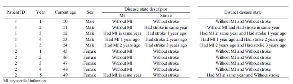
- The dataset typically requires calculating cost for discrete time periods. For instance, if you have claims data, you may have information on cost by date, but for analytic purposes may want to have a dataset with cost information by person (rows) with the columns being the cost by year (or month). Alternatively, you could create the unit of observation to be the person-year (or person-month) and each row would be a separate person-year record.
- Next, one must specify the disease states. In each time period, the person is assigned to a disease state. Challenges include determining how granular to make the states (e.g. just MI vs timing since MI) and how to handle multi-state scenarios.
- When data are censored one can (i) add a covariate to indicate data are censored or (ii) exclude observations with partial data. If cost data are missing (but the patient is not otherwise censored), multiple imputation methods may be used. Forming the time periods of analysis requires mapping to the decision model’s cycle length, handling censoring appropriately, and potentially transforming data.
- A sample data set is shown below.
Step 2: Model selection:
- The paper recommends using a two-part model with a generalized linear model (GLM) framework, since OLS assumptions around normality and homoscedasticity in the residuals are often violated.
- With the GLM, the expected value of cost is transformed non-linearly, as shown in the formula below. You are required to estimate both a link function and the distribution of the error term. “The most popular ones (combinations of link function and distribution) for healthcare costs are linear regression (identity link with Gaussian distribution) and Gamma regression with a natural logarithm link.)
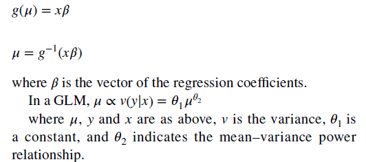
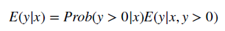
- To combine the GLM with a two-part model, one simply estimate the equation above on all positive values and then calculates a logit or probit model for the likelihood an individual has positive cost.
Step 3: Selecting the final model.
- Model selection first must consider which covariates are included in the regression which can be obtained by stepwise selection using a pre-specified statistical significance. However this can result in over fitting. Alternative covariate selection techniques include bootstrapping stepwise selection and penalized techniques (e.g. least angle selection and shrinkage operator, LASSO). Interactions between covariates could also be considered.
- Overall fit can be evaluated using the mean error, mean absolute error and root mean squared error (the last is most commonly used). Better fitting models have smaller errors.
Step 4: Model prediction
- While predicted cost are easy to do, the impact of disease state on cost is more complex. The authors recommend the following:
For a one-part non-linear model or a two-part model, marginal effects can be derived using recycled prediction. It includes the following two steps: (1) run two scenarios across the target population by setting the disease state of interest to be (a) present (e.g. recurrent cancer) or (b) absent (e.g. no cancer recurrence); (2) calculate the difference in mean costs between the two scenarios. Standard errors of the mean difference can be estimated using bootstrapping.
The authors also provide an illustrative example applying this approach to modeling hospital cost associated with cardiovascular events in the UK. The authors also provide the sample code in R as well and you can download that here.